MINI2P Distortion Detection

The MINI2P device in ScanImage represents a MINI2P head-mounted two-photon microscope. Because the MINI2P’s raster scanning has distortion that varies with FastZ depth, ScanImage provides a calibration workflow that measures the distortion and applies a per-depth geometric correction to acquired images.

Note

the distortion detection and correction workflow requires the MATLAB Image Processing Toolbox for interactive anchor-point alignment.

This document walks through:

1. What the MINI2P device does

2. One-time device configuration

3. Running the distortion-detection workflow

4. Applying the resulting transform to live display and to saved TIFFs

The process is documented imaging a grid slide slightly rotated relative to scanner axes with a confocal microscope, but the workflow is the same for calibrating a MINI2P itself.

What the MINI2P device does

The MINI2P dabs.mini2p.MINI2P device ties a calibration dataset (a set of geometric transforms, one per calibrated FastZ depth) to a specific scope and objective. Once configured, the device can:

• Store metadata about the physical scope (system name, scope name, objective) so calibrations are traceable to the hardware they were measured on.

• Correct the live display of any scanner paired with it by warping each live frame with the transform calibrated for the FastZ depth nearest the current viewport Z.

• Correct saved TIFFs after acquisition, either on demand or automatically, by spawning a background MATLAB instance that runs the correction and writes *_distcorrected.tif files alongside the originals.

The calibration itself is produced by the Mini2P Distortion Detection GUI. It saves a .mat file containing a cell array of per-Z transforms (the Transform Matrix file), which the MINI2P device loads on demand.

One-time device configuration

Open Resources → Mini2P to reach the MINI2P configuration page.

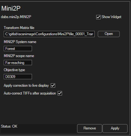
Required fields:

Transform Matrix file

Full path to the .mat file produced by the distortion-detection workflow. You can leave this blank at first and populate it after you run the workflow — the workflow itself offers to set this path for you after it saves.

MINI2P System name / MINI2P scope name / Objective type

Free-form identifiers. These are embedded in any transform .mat you save and in the headers of any TIFF you correct, so you can trace a corrected dataset back to the hardware that produced it.

Optional behavior checkboxes:

Apply correction to live display

If checked, any scanner paired with this MINI2P will have its live-display frames warped in real time using the transform for the Z nearest the current viewport Z.

Warning

Warping each frame dominates the display execution queue. At high frame rates this can noticeably slow the live display and may drop display frames (acquisition itself is unaffected). Disable this if your display slows.

Auto-correct TIFFs after acquisition

If checked, each time a ScanImage acquisition finishes, a background MATLAB instance is launched to run distortion correction on the TIFFs that were just written. This keeps the main ScanImage MATLAB responsive during what can be a slow correction pass.

Warning

The corrected TIFF has pixels rearranged from the original, thus the integrity of the data is slightly compromised by interpolation. The original, uncorrected TIFFs are unaffected and retain the raw pixel values. Use the corrected TIFFs for visualization, spatial analysis, and/or presentation.

Pairing a scanner with the MINI2P device

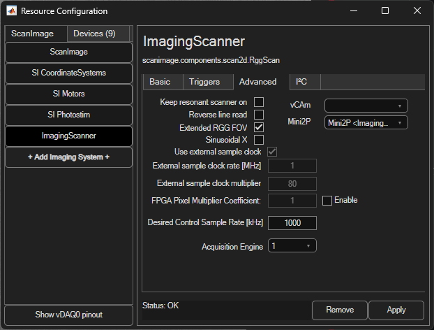
Live-display correction only fires for scanners paired to the MINI2P device. For RggScan scanners, open the scanner’s configuration page, go to the Advanced tab, and pick the MINI2P device from the Mini2P dropdown.

Running the distortion-detection workflow

From the Mini2P device’s widget, click Distortion Detection. The GUI walks you through five numbered steps. While the GUI is open, the MINI2P’s live-display correction is temporarily disabled and restored when you close the GUI, so what you see in the viewport during calibration is the raw, uncorrected image.

Step 1 — Image the grid

Mount a distortion grid slide to image. Confirm the System Name, Scope Name and Objective Type fields in the GUI match the hardware you are calibrating (they default to whatever the MINI2P device was configured with).

Click Focus to start a focus acquisition. Use the ▲ / ▼ buttons in the Image the Grid block to move only the Z-stage (FastZ stays put) until the grid is clearly visible.

The Tip: Set Averaging button turns on frame averaging; the grid is usually easier to align against a smoothed image.

Step 2 — Set coarse scaling

Two numbers to set here:

Real Grid Spacing

The physical spacing between grid lines on your slide, in micrometers. This is the ground-truth calibration distance.

Coarse Scaling [µm / °]

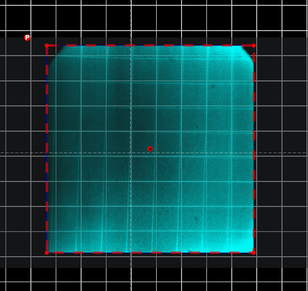
Bound to hSI.objectiveResolution. Adjust it until the virtual grid drawn in the viewport roughly matches the period of the imaged grid.

Tip: Ctrl+scroll in the viewport changes the live-image transparency, which makes it much easier to judge whether the virtual and imaged grids are in scale.

The Offset Sample Space Grid arrows shift the sample-space zero so the virtual grid points line up with visible intersections of the imaged grid.

Note

You may need adjust the y-axis scaling of the scanner at zoom = 1× to get closer to a 1:1 aspect ratio which helps to get the initial coarse grid closer to the imaged grid. DO NOT adjust the y-axis scaling after you have completed step 3. If for some reason aspect ratio changes with zoom, the distortion correction will account for this.

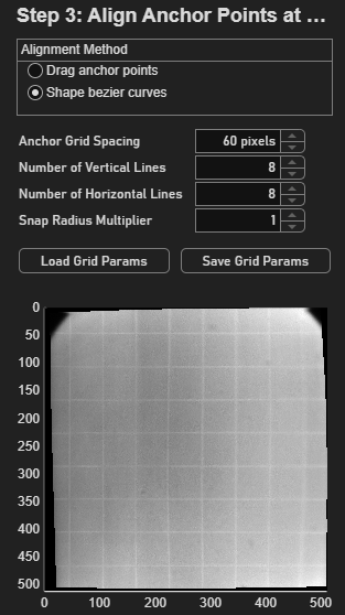
Step 3 — Align anchor points at the current depth

This is the per-depth calibration step. An anchor-point grid is overlaid on the viewport; move each anchor onto the imaged grid-line intersection it corresponds to, and the GUI builds the piecewise-linear transform from the resulting displacements.

Set Number of Vertical Lines, Number of Horizontal Lines and Anchor Grid Spacing (pixels) so the overlay approximately matches the imaged grid before you start dragging. Changing these spinners after you have dragged points will reset the overlay and discard your work.

You then have two alignment methods (selectable in the Alignment Method radio group):

Drag anchor points

Click and drag each individual anchor dot onto an intersection. Left- clicking near a point also snaps it to the mouse cursor if within Snap Radius Multiplier × Anchor Grid Spacing.

Shape bezier curves

Each grid line is represented by a cubic bezier; you drag the bezier endpoints and tangent handles to trace the curved grid lines, and the anchor points are computed from intersections of the bezier curves. This is usually much faster than per-point dragging for several grid lines, and you need to do the calibration for several depths.

Note

As the anchor points are computed from the bezier curves’ intersections, you will need to take care to drag the endpoints past the outermost grid lines to get a full set of anchor points covering the field of view.

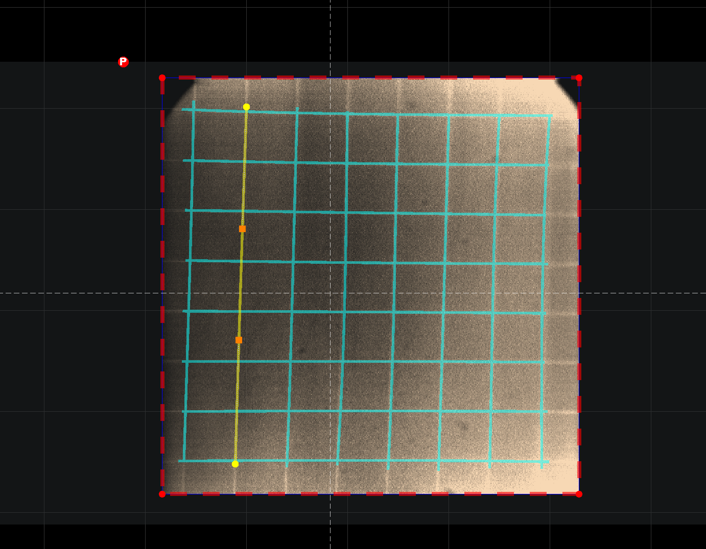
You can switch between methods at any time, and the anchor points are preserved across methods, so if you try bezier curves and it’s actually difficult to get a good fit, you can switch to dragging individual points without losing your work.

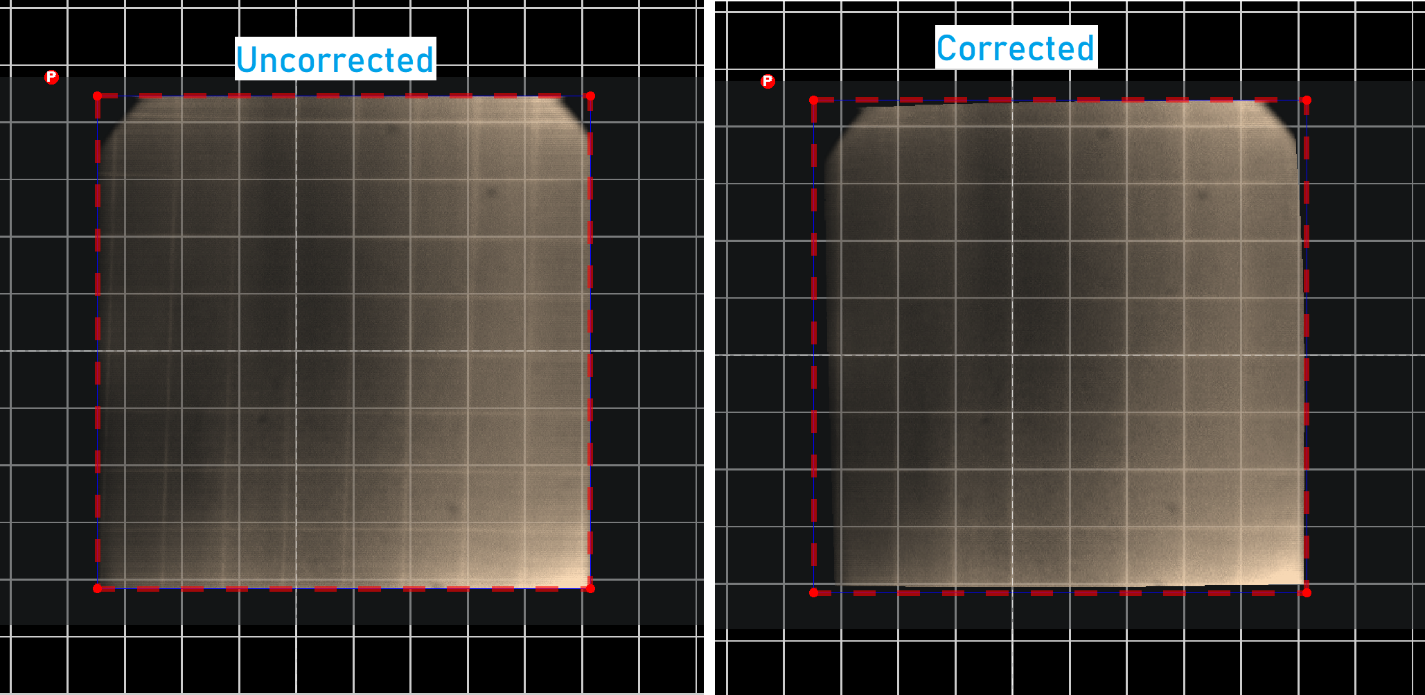
The preview axes in the GUI show the warped image in real time so you can see whether the correction flattens the grid.

Step 4 — Record this depth and advance to the next

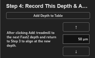
Once the anchor points or bezier curves are settled over the imaged grid, click Add Depth to Table. The current FastZ position becomes a new row in the Z table, with the current transform attached.

If you click the review button from stage 5, you can see red dots overlaid on the preview axes. If they are all lined up with the grid intersections, then the transform is doing a good job of correcting the distortion at this depth. If not, you can go back and adjust the anchor points or bezier curves to improve the fit before moving on to the next depth.

Note

Don’t move the stage laterally between depths.

Then use the Treadmill ▲ / ▼ arrows to move to the next FastZ depth you want to calibrate. Treadmill steps move the FastZ and the Z-stage in opposite directions, so the imaging plane stays at the same depth relative to the sample while the FastZ shifts to a new calibration point.

Return to Step 3 and re-align the anchor points for the new depth. Repeat across the full FastZ travel range you care about.

Step 5 — Save the full transform set

Click Save Transform Set to write a timestamped Transform Matrix .mat file to the current scan’s log directory. The file name encodes the scope name, zoom, and timestamp, so multiple calibrations on the same system remain distinguishable.

After saving, the GUI asks whether to set the MINI2P device’s Transform Matrix file to the one you just saved. Answer Yes to make the new calibration the active one. Any paired scanner with live-display correction enabled will then start using the new transforms immediately.

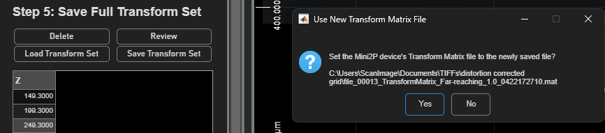
Review / Delete / Load buttons

• Review loads the transform for the Z currently selected in the table back into the anchor-point editor, so you can touch up a single depth without redoing the whole set.

• Delete removes the selected depth from the table.

• Load Transform Set loads an existing Transform Matrix .mat back into the GUI for further editing.

Applying the calibration to acquired data

Once a Transform Matrix file is set on the MINI2P device, you have three ways to use it.

Live display

Enable Apply correction to live display on the MINI2P configuration page. While acquiring, each live frame for any paired scanner is warped using the transform for the Z nearest the current viewport Z.

On-demand batch correction

Click the Distortion Correction button on the MINI2P device’s widget to run correction on a batch of saved TIFFs. The GUI prompts for a folder of TIFFs and runs the correction, writing <name>_distcorrected.tif alongside each input file. A foreground waitbar shows progress.

TIFFs that already have a SI.Custom.MINI2P header are skipped, so re-running on a mixed folder is safe.

Automatic correction after each acquisition

Enable Auto-correct TIFFs after acquisition on the MINI2P configuration page. When an acquisition finishes, the MINI2P device launches a background MATLAB instance to run on the TIF logging directory.

Because the work runs in a separate MATLAB, it does not tie up the foreground MATLAB’s execution queue — acquisition, display, and user interaction continue normally.

Troubleshooting

“Transform matrix file not found” in the log after an acquisition.

The MINI2P device’s transformMatrixDirectory points at a path that no longer exists. Either re-run Step 5 and accept the prompt, or update the path manually on the MINI2P configuration page.

Live display correction noticeably slows acquisition display.

Expected at high frame rates relative to the system’s capabilities. Disable live correction during imaging and use auto-correction or on-demand batch correction instead.

Auto-correction silently does nothing.

The background MATLAB instance’s errors are not visible in the foreground. Check that the Transform Matrix file exists.