SLM Diffraction Efficiency Calibration

As a diffraction-limited point projected by an SLM is steered farther away from the SLM’s zero order spot, the brightness of the point falls off. The exact profile of the fall off depends on multiple factors such as the accuracy of the SLM LUT and the alignment of the microscope. For optogenetic experiments, the varying intensity poses a challenge, as the cells should be illuminated with a known intensity. To overcome this challenge, ScanImage® includes tools to map the diffraction efficiency of the SLM over a 3D field of view.

ScanImage provides two ways to measure this map:

• a substage-camera method, which records the SLM’s projected spots directly with a camera below the sample, and

• a camera-free method (Simple SLM Diffraction Efficiency), which reads the efficiency out of images the SLM itself scans of a uniform fluorescent sample.

Both write the same per-rig diffraction-efficiency interpolant (hSlmScan.hSlm.hCSDiffractionEfficiency), which replaces the analytical sinc² fallback. During a photostimulation experiment the calibration is used to adjust the global laser power and the per-point intensity weights of the holographic points for even illumination.

Launching the calibration

Both calibration utilities are launched from the Alignment Tab. Under Alignments, the SLM Efficiency Calibration / Simple SLM Diffraction Efficiency button row opens the substage-camera GUI (scanimage.gui.align.SlmEfficiencyCalibrationGui) and the camera-free GUI (scanimage.gui.align.SimpleSLMDiffractionEfficiencyGui) respectively. The button row turns green once a diffraction-efficiency calibration has been applied by either method; the adjacent Reset button clears it.

Warning

If you use the Apply diffraction efficiency to power control (see SLM Imaging controls), turn it off before acquiring calibration data — otherwise the beam power is already being corrected during the measurement and the calibration will be wrong.

Method A — Substage Camera

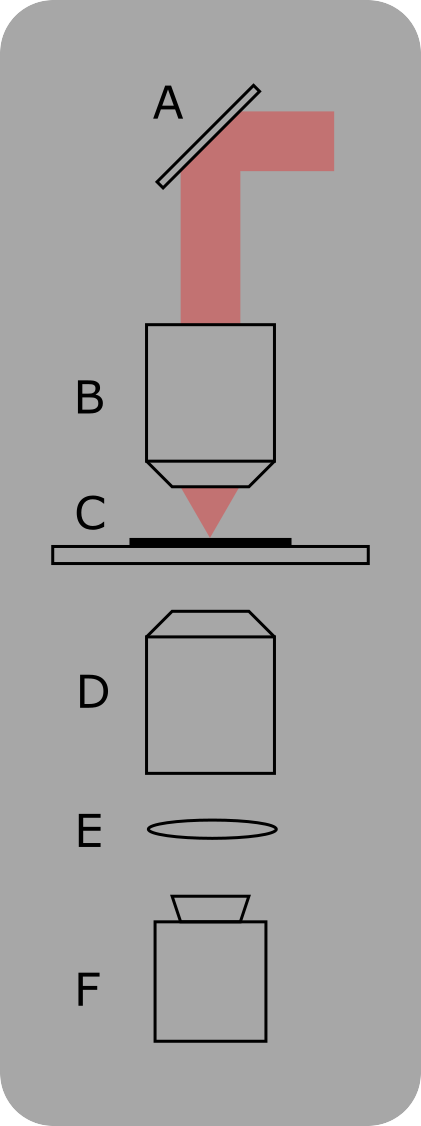
Substage Camera Setup

ScanImage:

A: SLM

B: Imaging objective

C: Thin fluorescent film on microscope slide

D: Camera objective

E: Camera tube lens and filter to remove excitation light

F: Camera

A homogeneous, thin-film fluorescent sample is positioned under the microscope. The SLM illuminates the sample at a given X/Y position and sweeps the Z focus through the sample, while the camera records an image for each Z position to form a point spread function. The sample is then moved to a different Z position by a stage, and the process is repeated until a sufficient number of points in the 3D field of view are surveyed. A polynomial function is then fit to the XYZ-intensity values.

Note

See the Cameras documentation page to get a list of supported cameras in ScanImage.

The SLM Efficiency Calibration GUI groups its controls into panels — Configuration Points, the calibration-point table, a Selected Calibration Point detail view, Status, Camera, SLM Calibration, and ScanImage.

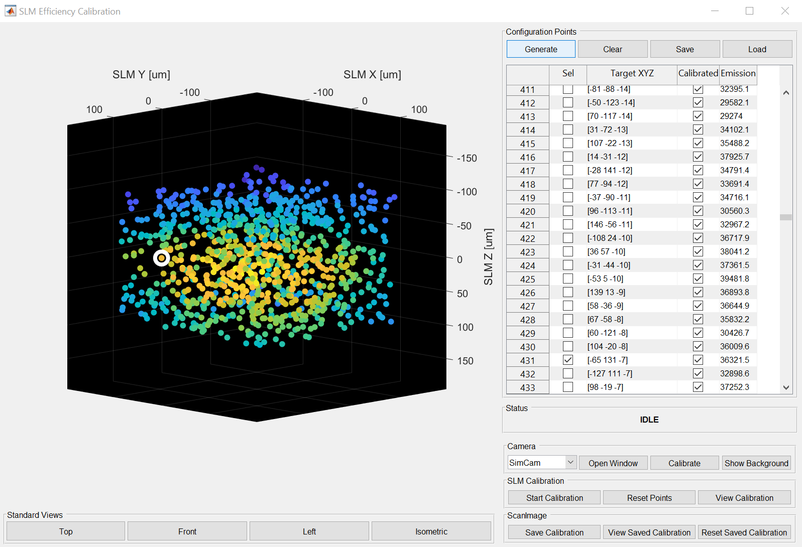
Calibration steps

1. Calibrate Camera

   The camera is used for intensity calibration. Dark current, static pixel offsets and dead pixels need to be calibrated before the intensity measurement. In the Camera panel, press Camera Tab to start the camera and confirm it is aligned to the imaging scanner and set so the brightest spot does not saturate. Then ensure no light reaches the camera sensor and press Calibrate Camera so the background noise can be subtracted from incoming samples.

2. Generate the calibration point cloud

   In the Configuration Points panel press Generate. The dialogs let you configure and generate a cloud of calibration points within the 3D volume — the number of points and their extent in XYZ. Points can be saved/loaded with Save / Load and cleared with Clear. If a zero-order beam block is painted into the SLM (see Zero-Order Beam Block), points that fall in the block are dropped from the generated set automatically.

3. Run the calibration

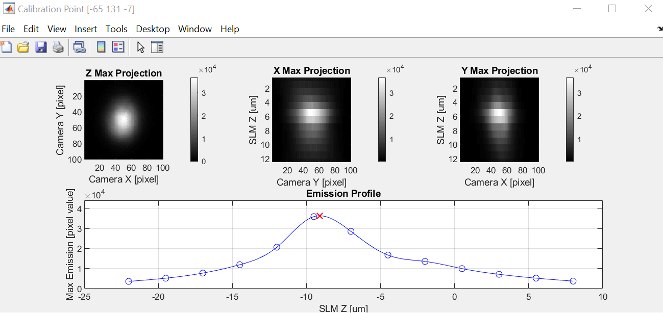
   In the SLM Calibration panel press Start Calibration. The calibration can use a motorized stage or a FastZ actuator. The first two points in the cloud need to be found manually by moving the FastZ / stage; the remaining points are calibrated automatically. Selecting a calibrated row in the table shows its Z/X/Y max projections and emission profile in the Selected Calibration Point panel. Reset Points clears the per-point results.

4. Inspect and save

   Press View Calibration to explore the fitted polynomial — drag the red cursor lines to move through the volume. If the calibration is satisfactory, in the ScanImage panel press Save Diffraction Efficiency to synthesize the data into the 3D interpolant. Optionally press Save Z Calibration to correct for field-curvature effects on a per-point basis. View Saved / View Saved Z visualize a prior calibration, and Reset Saved / Reset Saved Z return the calibration to a naive state.

Method B — Simple SLM Diffraction Efficiency (camera-free)

The substage-camera method requires a camera assembly below the sample. The Simple SLM Diffraction Efficiency method needs no camera: because SlmScan forms an image by pointing the SLM at one deflection per pixel, an image of a uniform fluorescent sample directly encodes the diffraction efficiency at each deflection angle. A thick fluorescent slide or a fluorescein bath provides the uniform sample.

Open the GUI from the Alignment Tab → Simple SLM Diffraction Efficiency. It presents a guided, top-to-bottom workflow:

1. Find the sample. Mount a thick fluorescent slide or fluorescein bath under the objective. Press Start Focus and pick the measurement channel from the dropdown.

2. Move the stage to the fluorescent layer. Using the ↑/↓ buttons (with the µm step field), move the stage only until the fluorescent layer is in focus. Press Set Z of Interest to zero the sample coordinates and pin a context image at this depth.

3. Window the signal. Press Open Signal Conditioning Tab and set the virtual-channel window so the collected PMT signal is masked to just the fluorescent emission between laser pulses.

4. Step through SLM depths (treadmill). Use the ↑/↓ buttons (with the µm step field) to step the SLM imaging depth. Each step moves the stage an equal and opposite amount, so the fluorescent layer stays in focus while the SLM refocuses through it. The live SLM Imaging Depth label tracks the current depth.

5. Acquire and accumulate. Press Set Resolution & Field Size to open the Single Scanfield panel — use equal pixels-per-line and lines-per-frame (the analysis requires a square frame). Then:

   1. Press Capture Reference (mirror SLM) once. With the zero-order beam block removed, this mirrors the SLM (flat phase mask → all power to zero order, i.e. efficiency = 1), briefly turns the beam on at the acquisition power, measures the full-power signal, and turns the beam off. This fixed reference makes the efficiency absolute and comparable across depths. The Reference label reports the captured value.

   2. At each SLM depth, press Start Focus / Grab Frame, then Add Calibration Point. The efficiency at each pixel is computed from the acquired frame as sqrt(signal / reference) (two-photon fluorescence scales as power², floored at 0.02). The depth(s) calibrated label increments.

   3. Repeat steps 4–5b across several SLM depths to span the working range.

   4. Press Apply Calibration to build the 3D diffraction-efficiency interpolant from all accumulated depths and write it to the SLM. Reset discards the accumulated points.

Zero-Order Beam Block

Many SLM photostimulation rigs place a physical block (e.g. a small metal disk) at the Fourier-plane focus to absorb the un-diffracted zero order. That region of the SLM’s field delivers no usable light, so it should be excluded from both calibration measurements and stimulation targets. ScanImage tracks the block as a mask in SLM-native XY (SlmScan.zeroOrderBlockMask, a 256×256 grid) that is saved with the scanner’s class data and applied live.

Painting the block. With the diffraction-efficiency surface visible in the Viewport, right-click it and choose Paint Zero Order Block. This starts an inline paint tool (ZeroOrderBlockPaintTool):

• Left-drag paints the blocked region; right-drag erases.

• The tool’s context menu offers Stop Painting Zero Order Block and Clear All; pressing Esc also stops painting.

Filling from a calibration. In the substage-camera GUI’s SLM Calibration panel, Fill Zero Order Block treats calibration points whose efficiency is at or below a prompted threshold as block locations and paints disks (of a prompted fill radius) at those points into the mask.

Once painted, generated calibration point sets skip any point that falls in a blocked cell, so the block region is neither measured nor targeted.

SLM Imaging controls

When a SlmScan is the active scanner, the Scan tab shows an SLM Imaging panel (scanimage.gui.SlmImagingGui) with the imaging controls relevant to these calibrations:

Control	Meaning
Imaging Depth [µm]	Z of the plane the SLM scans (the SLM defocus from the objective focal plane). This is the depth the camera-free treadmill steps; it is independent of the SLM park position.
Pixel Dwell Time [ms]	The data-acquisition window collected per SLM pixel.
Dwell [laser pulses]	The dwell expressed in laser pulses (dwell × laser repetition rate). Editable only when the acquisition is synchronized to the laser (vDAQ digitizer clock PLL locked); grayed out otherwise.
Apply diffraction efficiency to power	When enabled, per-pixel beam power is scaled by 1/efficiency (clamped to each beam’s power-fraction limit) to flatten excitation across the SLM field. The panel turns yellow with a caution note while this is active.

Warning

Apply diffraction efficiency to power must be off while acquiring data for either diffraction-efficiency calibration. If it is on, the per-pixel power is already corrected during the measurement, so the acquired image no longer reflects the raw diffraction efficiency and the resulting calibration is invalid.