SLM Photostim Calibration and Alignment
Phase LUT Calibration
SLMs take pixels from bitmaps and convert them to phase shifts. Ideally, each pixel’s phase shift would map linearly from 0 to 255. In reality, we must determine the actual relation.
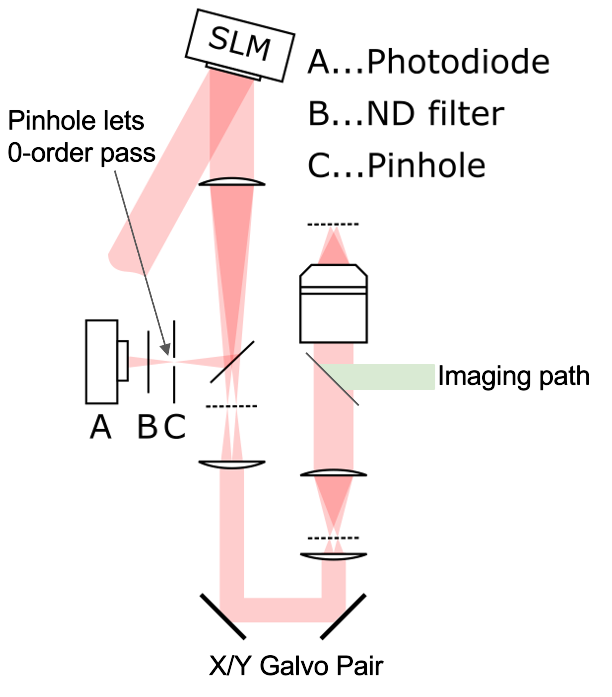
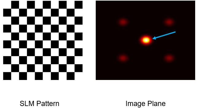
To calibrate the phase mask, a checkerboard phase mask pattern is applied to the SLM and every other checker square is swept through pixel value range [0, 255] while the others are held constant. At the same time, the intensity of the zero order spot is measured with a photodetector (read through an analog-input channel) as energy is diverted to higher order spots. The largest swing in measured zero order intensity while sweeping pixel values is used to map pixel values to phase.
The calibration is performed in the SLM LUT Calibration GUI
(scanimage.gui.align.SlmLutCalibrationGui), launched from the
Alignment Tab under Characterizations → SLM LUT Calibration. No camera
is required — the diffracted intensity is read back through a photodetector
wired to an analog-input channel.
The GUI has a Pattern Controls panel over two plots:
SLM Phase Response — measured intensity versus the swept checker pixel value.
SLM LUT — the resulting pixel-value ↔ phase curve.
Workflow:
Set the Pattern Controls parameters (table below) and pick the Measurement Channel (the analog-input resource the photodetector is wired to).
If beam modulators are present, set their power fraction so the SLM is illuminated when prompted.
Press Measure. ScanImage points the SLM to zero order, sweeps the checker pattern through the pixel-value range, and reads the diffracted intensity back through the selected channel. The response appears on the SLM Phase Response plot.
Drag the two red markers along the response curve to bound the monotonic portion used for the fit (a red diamond marks the detected peak). The SLM LUT plot updates live: the raw fit is drawn in blue, and — if Polynomial Degree > 0 — the polynomial-smoothed LUT is overlaid in red.
Press Save LUT to commit the wavelength and the fitted LUT to the SLM scanner.
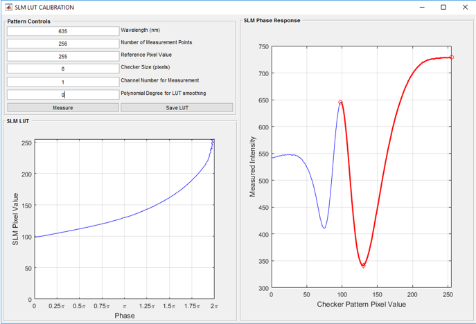
Wavelength (nm) |
The wavelength of the stimulation laser |
Number of measurement points |
The total number of total phase masks from the checkerboard pattern mask to the zeroed phase mask |
Reference Pixel value |
The pixel value of the checker squares whose phase remains the same throughout (defaults to the maximum value the SLM accepts, e.g. 255 for an 8-bit device) |
Checker Size Pixels |
The side length of each of the checker squares |
Measurement Channel |
The analog-input channel the photodetector is read through to measure the brightness of the zero order spot |
Polynomial Degree for LUT smoothing |
A polynomial curve can be fitted to the SLM Pixel Value vs Phase plot. A value of zero gives no polynomial fitting. |
SLM Flatness Correction
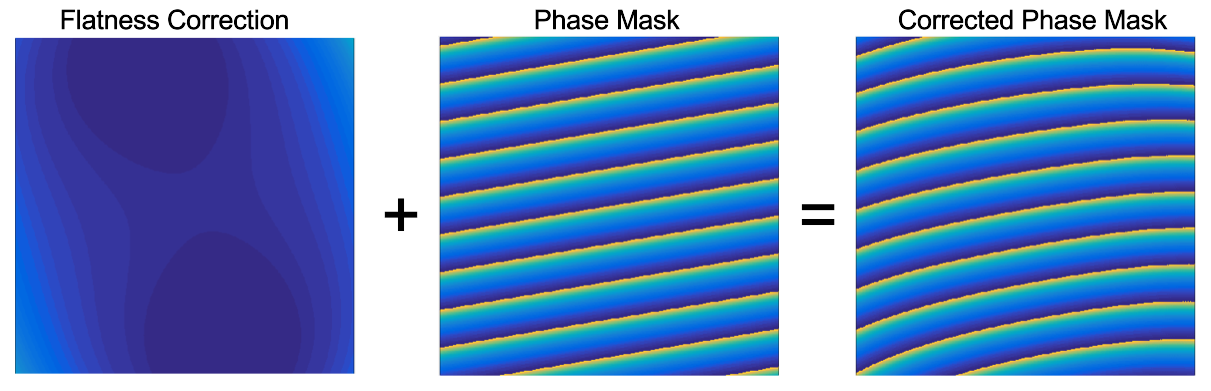
Wafer polishing of the SLM introduces a slight dome shape. To correct for this, a flatness correction file is provided by the manufacturer. The correction is wavelength dependent.
Spatial Alignment
All of the spatial alignment for the SLM happens through the SLM Spatial Alignment
GUI (scanimage.gui.align.SlmSpatialAlignmentGui), which is launched from the
Alignment Tab. The GUI bundles:
A Z Alignment panel that owns the LUT
hSlmScan.hCSSlmNative.fromParentLutEntries. Each LUT entry maps a focal depthz_ScannerOffset(in µm, X axis) to an SLM vergencezto(in diopters, Y axis), along with a 2D affine for the lateral correction at that depth.A Coarse Adjustment panel (
SlmAffineAdjustmentPanel) that nudges the 2D affine of the LUT entry nearest the currently targeted Z (within 1 µm).A tabbed XY-alignment area with three refinement workflows that write the 2D affine for the same entry:
Substage Camera — overlays a grid of SLM-aimed laser spots on a live camera image.
Burn Spots — burns a grid of holes into a fluorescent slide with the stim laser, then matches the imaging-scanner picture of those holes to the grid the SLM was commanded to.
Motion Detection — deflects a single SLM focal point laterally and reads the resulting offset, either by automated motion estimation or by manually overlaying the live (deflected) image onto a pinned reference. Useful when no camera is available and a hole-burning slide is undesirable.
Because the lateral correction is stored per Z entry, the workflow below deliberately defers any XY tweaks to the depth at which they are being viewed.
Step 1 — Align the linear scanner to the imaging scanner
If the SLM is relayed onto a linear scanner that is paired with a separate imaging scanner, the two scanners need to be brought into the same coordinate system before any SLM-specific alignment is meaningful.
The stimulation path and the imaging path do not in general share the same focal depth in the sample — at the SLM’s zero phase mask the two image planes can easily be tens of microns apart. Aligning the linear scanner to the imaging scanner therefore requires two passes: a Z calibration first, then a lateral one.
1a. Match the focal depths at z = 0
The Z mismatch is absorbed by the hCSScannerOffset LUT entry at
zfrom = 0. Adjust this entry’s zto so the linear-scanner image plane
coincides with the imaging-scanner image plane. Do not touch the 2D
affine on this entry yet.
Sample: a thin layer of yellow highlighter on a glass slide. For a water-dipping objective, drop a coverslip on top of the highlighter before adding the water droplet, and don’t add so much water that it spills past the edge of the coverslip onto the highlighter underneath.
Park the FastZ at target position 0 on the linear scanner’s FastZ device.
Focus with the imaging scanner.
Step the Z-stage until the histogram of the image data is at its maximum value — that’s the depth where the highlighter layer is in focus through the imaging path.
Zero the sample relative coordinate system at this depth. Optionally pin the current imaging-scanner frame to the viewport background for reference.
Switch imaging to the linear scanner paired with the SLM (SlmScan’s paired linear scanner).
Scan with the linear scanner and, in the Z Alignment panel, adjust the
ztofor thehCSScannerOffsetLUT entry atzfrom = 0until the histogram is once again at its maximum mean pixel value across the frame — the two image planes now coincide. If there is slight non-uniformity in the highlighter layer or a small tilt of the sample, overlay the live image on the pinned reference at reduced opacity to compare them directly.Tip
With the cursor inside the viewport, Ctrl + scroll adjusts the alpha of the live image, making it easy to fade between the live linear-scanner frame and the pinned imaging-scanner reference.
1b. Laterally align the linear scanner to the imaging scanner
Once the focal planes coincide, swap to a thin sample with structure that both paths can resolve (a thin pollen slide or fluorescent beads on a coverslip works well).
Open the Alignment Tab and bring up the
Scanner-to-Reference alignment tool
(scanimage.gui.viewport.tools.liveDisplay.ScannerToRefAlignmentTool).
The tool freezes a copy of the reference scanner’s pinned image plus any
visible ROI and scanfield overlays in scanner space, so dragging fixed
points moves the live image relative to that frozen reference. Follow the
standard Scanner-to-Scanner Alignment workflow to drag the linear-scanner
image onto the reference image.
The right-click context menu on the tool also offers:
Clear transform at current z — remove the LUT entry of
hCSZAffineLutat the current Z, falling back to whatever the LUT interpolation says.Reset transform at current z — set the LUT entry at the current Z to the identity (or insert one if none exists within 1 µm).
When the Apply menu item is selected, the new transform is committed to
hCSZAffineLut at the viewport’s current Z.
Step 2 — Coarse lateral alignment at z = 0
With the linear scanner now aligned to the imaging scanner, the SLM’s own lateral alignment can be tackled. Start at the calibrated z = 0 LUT entry (scanner offset = 0 µm). The intent is to take out the bulk of the mismatch first with the simple coarse-adjustment controls, then refine with the camera or hole-burning workflow.
2a. Coarse adjustment with the SlmAffineAdjustmentPanel
The Coarse Adjustment panel (SlmAffineAdjustmentPanel) writes directly
to the 2D affine of the LUT entry of hCSSlmNative.fromParentLutEntries
nearest the currently targeted Z (within 1 µm); if no entry is within
tolerance, an identity entry is created at the target Z first and then
nudged. The panel exposes four absolute fields and four nudge sliders:
Scale (%) — ratio of galvo°/SLM° × 100. The expected value comes from the SLM-to-galvo relay transverse magnification:
scale ≈ 100 × f1 / f2
where f1 is the focal length of the relay lens adjacent to the SLM and f2 the one adjacent to the galvos. For a 100 mm / 200 mm pair the panel should land near 50 %.
X Offset / Y Offset — translation in SLM-native coordinates. The
-/+buttons step by the slider’s percentage ofhSlm.nativeRangeXYZ(i.e. an XY shift expressed as a fraction of the SLM’s full deflection range).Rotation (°) — rotation around the optical axis.
Invert X / Invert Y — flip the corresponding axis (handy when the relay or a downstream mirror has produced an unexpected handedness).
Reset Adjustments At This Z — restore the LUT entry’s affine to the identity (the Z mapping itself is preserved).
Type a value into one of the absolute edit fields and press Enter, or use
the slider + -/+ buttons to nudge. Each click commits to
fromParentLutEntries and saves the coordinate systems.
For this step, the easiest sample is a layer of yellow highlighter on a glass slide, viewed through the substage camera. Park the SLM at z = 0, project a single point or a small grid, and use Scale / Offset / Rotation / Invert to walk the projected spot(s) onto the centre of the camera field — close enough that the refinement step below will converge.
2b. Refine with the substage-camera, burn-spots, or motion-detection workflow
After the coarse pass, pick one of the three tabbed workflows in the SLM Spatial Alignment GUI to compute and apply the refinement affine.
Substage Camera tab (SlmCameraAlignmentPanel)
Sample: yellow highlighter on a glass slide.
Press Start Camera to open the Camera Tab and begin live acquisition on the first configured substage camera.
Set the Grid lines and % FOV fields (defaults 5 lines, 0.6 of the SLM native range).
Press Project Grid to point the SLM at a grid of XY targets at the currently targeted
z_ScannerOffset(taken from the Z Alignment panel).Press Start Alignment to overlay the ideal grid on the live image via
SlmAlignByGrid. The default mode is bezier — drag the row and column curves (and the tangent handles at their endpoints) until the curve intersections coincide with the visible laser spots. Switch to drag swaps to per-point dragging if you prefer.Optionally press Detect Spots to auto-fit centroids (bright-polarity) to the projected spots.
Press Generate Alignment to solve a 2D affine via
pinvmapping the observed (dragged) ref-space positions back to the SLM-native targets. The new affine is left-composed with the existing LUT entry’s affine at this Z, or a new entry is created if none exists within the 1 µm tolerance.
Burn Spots tab (SlmBurnSpotsAlignmentPanel)
Sample: a fluorescent slide marked with permanent marker (Sharpie). The stim laser ablates the marker, leaving fluorescent bright spots in the imaging-scanner image.
Press Start Focus — the GUI switches the imaging system to the SLM’s paired linear scanner, sets the scan mode appropriately, and begins a focus acquisition.
Configure Grid lines, % FOV, Burn [um] (burn spot diameter), Power [%], Burn [s] (per-spot duration), and Pause [s].
Press Burn Holes. The panel closes the detection-path shutters, powers off the PMTs, fires the configured grid as an on-demand photostim ROI group, and then restores the prior shutter / PMT / photostim state. The XY grid is sized relative to the default imaging scanfield, scaled by % FOV.
Press Start Alignment, then drag the bezier curves (or individual markers, Switch to drag) so the curve intersections fall on the burn spots.
Optionally press Detect Spots — same auto-fit as the camera workflow, but with dark polarity.
Press Generate Alignment to commit the affine to the LUT entry at this Z. Burning requires a calibrated Z entry already in place, so this workflow is also usable as the refinement step at any other depth in step 4 below.
Motion Detection tab (SlmMotionDetectionPanel)
Sample: any thin sample with enough structure for the imaging scanner to resolve a single deflected SLM focal point (e.g. a pollen slide or beads). No camera is required. Rather than fitting a whole grid at once, this workflow records the lateral offset of one deflected point at a time and fits the affine from at least three such points.
The Alignment input dropdown selects how the offset is read:
Motion Estimation — ScanImage’s simple motion correction cross-correlates each live frame against a reference to measure the lateral offset automatically.
Manual Overlay — a fallback for when SLM defocus scales the live image (which breaks cross-correlation): the current frame is pinned as a reference and a live-image overlay tool is started, so you drag the live (deflected) image over the pinned reference and the overlay’s translation is taken as the offset.
Press Start Focus to begin a focus acquisition on the SLM’s paired linear scanner.
Press Start Alignment. This opens the Phase Mask Display so the SLM focal point can be deflected laterally. Motion Estimation enables motion correction; Manual Overlay pins the current frame and starts the image-overlay drag tool.
Deflect the SLM focal point laterally with the Phase Mask Display. In Manual Overlay, drag the live image back onto the pinned reference. Then press Add Alignment Point to record the current SLM deflection and its lateral offset. A minimum of three points is needed for a full affine; Reset Points clears them.
Press Finish Alignment to fit the full lateral affine and fill in the
affine2Dof the SLM’s existinghCSSlmNative.fromParentLutEntriesentry at the current depth. View Alignment Matrix prints the current LUT entries for inspection.
Note
Like the burn-spots workflow, Finish fills in an existing Z entry’s affine — it never creates one — so the SLM Z depth must already be calibrated (step 3) before finishing a Motion Detection alignment.
Step 3 — Calibrate SLM Z at several depths
Once the lateral alignment at z = 0 is good, sweep the SLM through Z and
record a vergence-vs-depth point at each of several focal offsets. This
populates the hSlmScan.hCSSlmNative.fromParentLutEntries LUT with the
zfrom / zto pairs that drive the SLM vergence used at runtime.
Sample: the same yellow highlighter on a glass slide.
The Z Alignment panel (SlmZAlignmentPanel) presents:
An axes with Z [µm] (scanner offset) on X and SLM vergence [diopter] on Y.
A blue marker for each calibrated entry; entries that also have a non-identity 2D affine are filled blue (hollow otherwise).
A red position marker showing the SLM’s currently commanded (Z, vergence) point.
Left / right arrows — scan the Z view (move the red marker in X) without writing to the LUT.
Up / down arrows — adjust the SLM vergence at the current Z and write/update a LUT entry there.
Goto Zero, Auto-fit, Reset LUT, and a Z [µm]: editable field with a ← Display Z button that syncs the field to the Viewport’s current focus-relative Z.
A Treadmill checkbox + dropdown. When enabled, every change in SLM
z_ScannerOffsetis paired with an equal-and-opposite move on the selected device (Z-stage, or one of the linear scanner’s FastZs) so the physical focal plane stays where it is while you hunt the SLM’s refocusing match. Jumps larger than 200 µm prompt for confirmation.
Workflow at each depth:
Choose the Z-stage / FastZ depth you want to calibrate (turn Treadmill on if you’d rather keep the physical focal plane fixed and walk the stage in response to SLM steps).
Use the up / down arrows to adjust the SLM vergence until the highlighter layer comes into focus in the imaging scanner.
Tip
Shift + scroll wheel over the axes zooms the Y axis (SLM vergence) centred on the red marker, letting you hunt vergence at arbitrary precision without overshooting the focus.
The LUT entry at this Z auto-updates as you nudge.
Repeat at several depths to span the working range. Right-clicking a point in the axes offers Goto, Delete, Reset XY alignment, Align XY at this Z, and Copy this XY alignment to other Zs.
Step 4 — Laterally align at each calibrated depth
The lateral correction can shift between Z entries because the SLM’s imaging through the optical train is not perfectly telecentric. Once Z is calibrated at several depths (step 3), revisit the lateral alignment at each of those entries.
For every calibrated Z:
In the Z Alignment panel, right-click the entry’s blue marker and choose Goto to drive the SLM there, then Align XY at this Z. This hands off to whichever XY-alignment tab is currently selected:
Substage Camera — restarts the camera if needed, projects the grid at this Z, and brings up the alignment tool.
Burn Spots — sets the burn target Z to this entry (you still need to press Burn Holes and Start Alignment yourself, since burning is destructive).
Motion Detection — does not take a Z target; once the SLM is parked at this depth via Goto, just run the Motion Detection workflow (steps above) and Finish writes the affine into this entry.
Run the chosen refinement workflow as in step 2b. The resulting affine is left-composed onto the existing entry at this Z.
Use the substage-camera workflow with highlighter-on-glass when a camera is available; use the burn-spots workflow with Sharpie-on-fluorescent-slide, or the motion-detection workflow with any structured thin sample, when only the imaging scanner is available. Calibrated entries with a non-identity 2D affine show as filled blue markers in the Z Alignment axes, so it’s easy to see at a glance which depths still need XY work.
Tip
If you’ve already produced a good affine at one Z and the optical train is roughly telecentric over the range of interest, right-click that entry and choose Copy this XY alignment to other Zs to bootstrap every other entry with the same affine. Then revisit each one only to the extent that residual error makes it worthwhile.