Offline Data Viewer

Frame Scanning Data
(Data from Boaz Mohar, Svoboda Lab, Janelia Research Institute)
The offline data viewer tool will open ScanImage data generated either in traditional frame scanning or arbitrary line scanning. Advanced imaging modes including stacks, fastZ, and multiple regions-of-interest (MROI) are supported. The tool allows you to easily create plots to show the change in fluorescence over time for a given pixel or area. For frame scanning, the tool also allows you to render 3D MROI data to a video or tiff file for easier downstream analysis.
Using the Offline Data Viewer
The offline data viewer can be launched by running the following command at the MATLAB command prompt:
>> sidataview
A prompt will appear for you to select a file. Once a file is selected, the data viewer will load. You can have multiple files open simultaneously in different windows by running the command again. The main window consists of three main views: the time slider control at the bottom, the image view on the right, and the plot view on the left.
Time Slider
Dragging the control on the time slider will update the data in the image view to show the data that was collected as the specified point in time. A red line will also appear in the plot view marking the same time point in the plot. If the plot view has been zoomed in, a yellow box in the time slider will appear indicating the region of time that is currently visible in the plot.
For viewing arbitrary line scanning data, the time slider view will also include a data map of the experiment. This view can be interpreted in the same way as the similar view in the live channel window during an arbitrary line scanning experiment. The horizontal axis of this map view corresponds to experiment time while the vertical axis corresponds to cycle phase. A vertical line in this map view represents all the data collected in one scan of arbitrary scan path. A horizontal line represents the fluorescence collected at a specific point in the path across all collected frames (cycles).
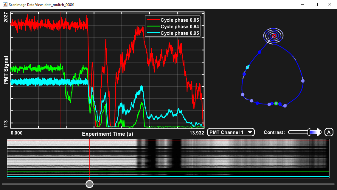
Line Scanning Data
Image View
The image view shows the data collected in the context of the overall field-of-view (FOV) where it was imaged. For frame scanning this is in the form of rectangular raster-scanned fields, while for arbitrary line scanning this is a path. The area can be panned by clicking and dragging with the mouse and zoomed with the scroll wheel. For volume data (slow stacks and fastZ) a selection appears at the bottom left of the image view to choose between 2D and 3D view. In 3D view, clicking and dragging while holding the SHIFT key on the keyboard orbits the data to change the viewing angle. In 2D mode a slider appears at the right hand side of the image view to select what Z is currently visible. The scroll wheel will traverse Z planes while the mouse is hovered over this slider. A text box above the slider can also be used to control the Z position. Beneath the text box, the “Current” checkbox can lock the Z position to the time position. When this is enabled, dragging the time control on the slider described in the previous section will cause the z position to move to the Z plane that was imaged at that time. This mode is enabled by default.
When viewing frame scanning data, the “…” button appears to the right of the view mode selection. This opens a view properties panel with additional options. The “Show Scanfield Borders” option allows enabling or disabling the blue box that indicates the shape of each ROI. “Enable Transparency” toggles transparency of dark pixels in each ROI. “Slice Spacing” will adjust the space between different z planes.
Plots can be created by clicking on the data. A single click will plot the data for a single pixel (or a single point along the path for arbitrary line scanning) over time. Clicking and dragging will create a plot that is spatially averaged over the selected region. Right click a plot point or region to remove the plot. For arbitrary line scanning you may also right click the area behind the path and add a context image. A context image can be loaded from a frame scanning data file collected with ScanImage.
The bottom right of the image view has a control for the image contrast, with sliders for the black and white levels. The “A” button will automatically adjust the contrast for the data currently visible. If the data being viewed was collected over multiple acquisition channels, a drop down selector will appear to the left of the contrast slider to allow selection between channels.
Plot View
The plot view is where plots created from the image view will appear. The vertical (PMT signal) scale limits of the plot view correspond to the contrast settings of the image view. Using the scroll wheel while hovering over the plot view will adjust the horizontal (time) plot limits. When the time scale has been zoomed in, a yellow box appears in the Time Slider view to indicate the visible time region. Right clicking on the plot view allows you to show or hide the plot legend as well as export plots to MATLAB for further manipulation. Right clicking a plot allows you to remove the plot from the view.
Rendering Frame Sequences
When working with multiple ROI data, the tiff format concatenates data collected from different ROIs vertically. While this is the most efficient way to store the data in real time, work is required to visualize it in the context of the ROI positions in the overall FOV. The Offline Data Viewer parses the ROI structure data saved in the tiff in order to show the data in the context of the actual ROI positions. If you desire to do further analysis of the data using another analysis tool, the Offline Data Viewer can render the data back to a tiff, but with the spatial information preserved. Alternatively, a 3D video of the data can be rendered to make a simple preview of the data.
To utilize the frame rendering feature, click the “Render Frame Sequence” button at the top of the image view. Select “2D” render type to render a tiff with each Z slice in a separate frame. For a 2D render, the aspect ratio of the rendered image is set automatically by the overall area needed to render all ROIs in the FOV. The pixel resolution can be modified or automatically set. If automatically set, the resolution is set to match the resolution that the ROIs were actually imaged at. Lowering the resolution will result in a lower file size but interpolated data points. Click the start button to proceed with the render.
For a 3D render, click the “configure” button to arrange the camera for how you want to see the data in the video. You can resize, pan, and orbit the data in the same manner as you can in the image view. This tool sets the aspect ratio of the video render. The actual pixel resolution can be set on the frame rendering panel. Finally, the quality setting can be used to trade off between file size and video quality.