Arbitrary Line Scanning
Arbitrary Line Scanning (ALS) is a premium feature in ScanImage that enables fast, high-resolution scanning along user-defined paths instead of raster scanning. This is especially useful in neuroscience and physiology experiments where the regions of interest (e.g., dendrites, axons, vessels) do not conform to rectangular imaging areas. With ALS, you can scan custom trajectories (lines, curves, loops) across your sample with precise control over timing, resolution, and intensity. The scan path can be designed in 2D or 3D, enabling use of a fast Z actuator for arbitrary volume scanning. In addition to recording fluorescence signals, the line scanning feature includes the ability to record and show in real-time the actual positions of the scan mirrors to ensure that they are accurately hitting the desired ROIs.
Use Cases
Measuring calcium transients along dendrites
Capturing signals along vessels
Tracking movement along axons
Fast temporal resolution, upwards of 200 Hz depending on the scan path, where raster scanning is too slow
Prerequisites and hardware requirements
ScanImage Premium License
Compatible scanner
Compatible DAQ hardware:
NI Galvo Galvo setup: In order to utilize the scan mirror position recording, an auxiliary DAQ must be present and the galvo position signals must be on a different DAQ than the photo-detector signals.
Proper system calibration
Up-to-date ScanImage installation
Step by Step Guide
To utilize arbitrary line scanning, select a linear scanning system as the active imaging system or select a linear scan mode for an RGG system on the scanner configuration tab interface, then add the Arbitrary Line Scan tab. A left pane and auxiliary panel will be brought up.. The Enable Arbitrary Line Scanning button can be toggled on so that the next acquisition will use arbitrary line scanning.
Add Reference Image
It is optional, but recommended to start with a context image in the viewport. This can be achieved by directly grabbing a live image or loading one from a presaved background.
Add ROIs
Before starting a scan, a scan path
must be configured. You can do so by selecting Add ROI to draw Rois, or Load ROI Group to load a previously saved Roi group.
Draw in the viewport
Selecting Add ROI will activate a tool in the viewport for drawing arbitrary line scanning ROIs,
allowing to draw one or multiple consecutive patterns.
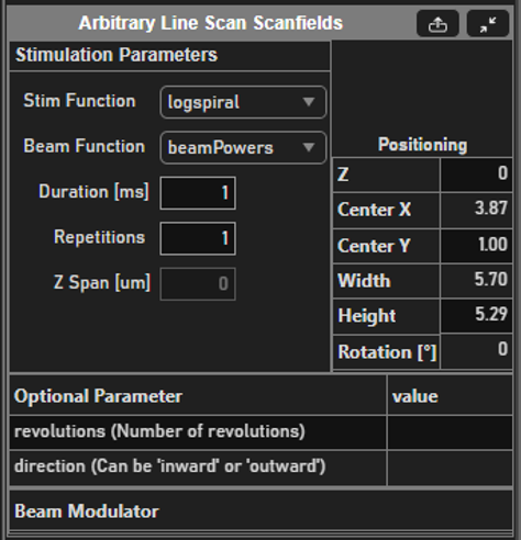
Select function and its parameters
If you are more familiar with photostimulation, the scan path is designed as a stimulus group, the same way photostimulation patterns are designed. Stimulus groups are a special kind of ROI group that define a parametric path instead of a 3D volume. A stimulus group is comprised of multiple ROIs that define a continuous sequential laser path. Stimulus groups allow complete freedom in designing the path for the laser to take. Best practices should be followed to ensure desired results. A stimulus pattern is comprised of a sequence of stimulus functions, each of which can be parameterized with:
Parametric function: The stimulus function can be chosen from a set of built in or custom stimulus functions
Position
Size
Rotation
Laser power
Number of repeats
Custom function parameters
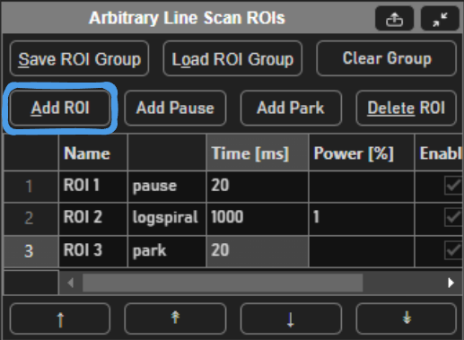
A typical stimulus pattern should consist of pause functions interleaved with stimulus functions at desired positions, as shown below:
Pause function
Sinesquare function
Pause function
Logspiral function
Pause function
Point function
Park function
The pauses between stimulations are important because the galvos require time to travel between ROIs. Without the pauses (or if the pauses are too short), the pockels cell will be open while the galvo is still traveling to the desired ROI, causing light exposure to the wrong part of the sample. If too large of a change in position is commanded without adequate transit time, or if the stimulus pattern is too demanding of performance from the galvos, the galvo controller may reset, causing a momentary loss of galvo position control. It is therefore important to carefully design the stimulus pattern to avoid this and test the pattern to make sure the results are desirable. By default, ScanImage will interleave drawn stimulus patterns with pauses and terminate the Roi group with a Park function.
Waypoints are a special stimulus function that can be very useful for designing a scan path. If there is a point you are interested in sampling data at, you could place a point stimulus function there. This would cause the scan mirrors to move to that point and stop there for the specified duration. It is much faster, however, to pass through the point without stopping, just exposing the beam over the point. This can be achieved using a waypoint function. Waypoints constrain the path to pass through the desired position with the beam exposed for the desired duration as the scan mirrors pass through the point.
If it is desired to create a custom stimulus function of a user-defined shape, please see the page on writing custom stimulus functions.
Editing the scan path
The controls in the Arbitrary Line Scan Rois tab can be used to reorder or remove functions. Select a stimulus function in the table or in the viewport to view its parameters in the arbitary line scan scanfields. One scan of the complete path is referred to as a cycle or frame. The Frame Rate on the scan tab interface indicates how fast cycles can be scanned (dictated by the total time duration of the path you have designed).
Executing a Line Scan
At this point you can start a FOCUS, GRAB, or LOOP from
the Acquisition Controls interface.
These operations function the same way they do for normal raster scanning.
A FOCUS will run the scan path continuously to display data only.
A GRAB will run the scan for the specified number of cycles and log
data to disk if logging is enabled. You can specify the number of cycles
to run by setting the number of frames to collect on the
Acquisition Controls interface.
A LOOP will execute multiple GRAB sessions.
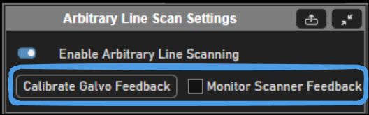
Verifying the Scan Path
Position feedback can be enabled to log to disk and show in real time the actual path scanned by the mirrors.Utilizing the Monitor Scanner Feedback on the Arbitrary Line Scan Settings tab is a good way to verify the galvos are able to follow the designed path. The prerequisite is that the galvos have feedback configured and are calibrated in ScanImage using the Calibrate Galvo Feedback button or directly from the galvo widget.
Note
Recording scanner feedback data for the Z actuator is not yet supported
Reading Line Scanning Data Files
The data is written to disk in multiple files to facilitate efficient processing. This helps enable higher sample rates due to low processing overhead. By default, each line scanning GRAB session will create 2 files:
[File name stem][File counter].meta.txt (Ex: filename_00001.meta.txt): Plain text file containing metadata describing the ScanImage® parameters and stimulus pattern used for the scan
[File name stem][File counter].pmt.dat (Ex: filename_00001.pmt.dat): Binary data file containing the collected fluorescence data
A third file is created if position monitoring is enabled
[File name stem][File counter].scnnr.dat (Ex: filename_00001.scnnr.dat): Binary data file containing the collected scanner position feedback data
ScanImage® includes a utility function to read these files and load the data into a convenient structure.
Using the ScanImage® Utility
The ScanImage® utility to load a data file can be called with the following signature:
1>> [header, pmtData, scannerPosData, roiGroup] = scanimage.util.readLineScanDataFiles(fileName)
The meta data and data files should exist in the same directory and fileName should be entered without the extension (ex: “filename_00001”). The return values are the following:
header: A hierarchical data structure containing the ScanImage parameters used when the data was collected as well as useful statistics about the total number of samples and frames collected and sample rate information. Reference the ScanImage API for more information about the contents of data log headers.
pmtData: A matrix of the collected fluorescence data organized by channel and frame. The size of the matrix is NxCxF where N is the number of samples per scan cycle, C is the number of channels, and F is the number of frames (cycles) collected. Index this array appropriately to extract the data you are interested in. To plot data collected during the 100th frame on channel 2, for instance, you could do the following:
1% squeeze is needed to remove the first dimension since it becomes singleton
2plot(squeeze(pmtData(:,2,100)));
To plot data at point 600 from channel 1 over every frame (ie a plot of how fluorescence at a single point is changing over time) you could do the following:
1% squeeze is needed to remove the third dimension since it becomes singleton
2plot(squeeze(pmtData(600,1,:)));
scannerPosData: If scanner position monitoring was on, a structure with a fields “G” and “Z” containing matrices for recorded scanner position data for scan mirrors and the Z actuator respectively. The size of the G matrix is Nx2xF where N is the number of data points per cycle and F is the number of frames collected. The columns correspond to the X and Y mirrors. The size of the Z matrix is Nx1xF where N is the number of data points per cycle and F is the number of frames collected. To plot the path of the X scan mirror collected during the 100th frame, for instance, you could do the following:
1% squeeze is needed to remove the first dimension since it becomes singleton
2plot(squeeze(scannerPosData.G(:,1,100)));
To plot the position of the Y scan mirror at point 600 from over every frame (ie a plot of the repeat-ability of scan mirror position at that point in the path) you could do the following:
1% squeeze is needed to remove the third dimension since it becomes singleton
2plot(squeeze(scannerPosData.G(600,2,:)));
roiGroup: A copy of the stimulation pattern that was used to collect the data. Reference the ScanImage API for more information about how to work with ROI Group objects.
Manually Decoding Data Files
If it is desired to write your own code to load the files (for instance if you need to perform analysis outside of MATLAB) the following provides information about how to read the files.
Metadata File: (Ex: filename_00001.meta.txt): This is a plain text file. If the option is enabled to store metadata in JSON format, there will be two JSON structures. The first will be a hierarchical data structure containing the ScanImage® parameters used when the data was collected. The second structure will be a data structure representing the stimulus pattern that defines the scan path used to collect the data. If the JSON option is not enabled, the ScanImage parameters will be written with “dot” syntax to represent the data sctructure, ie:
SI.hScan2D.sampleRate = 1.2e+08
In this case, the stimulation pattern info following the ScanImage parameter data will still be JSON. You can detect if the ScanImage data is stored as JSON by checking if the first character of the file it “{“.
Fluorescence Data File: (Ex: filename_00001.pmt.dat): This file contains raw binary data of samples written as signed 16-bit integers. The order that samples are written is:
[Channel 1 Sample 1, Channel 2 Sample 1, ..., Channel N Sample 1,
Channel 1 Sample 2, Channel 2 Sample 2, ..., Channel N Sample 2, ...,
Channel 1 Sample M, Channel 2 Sample M, ... Channel N Sample M]
where N is the number of channels and M is the number of samples per channel. The number of channels can be found in the header by counting the number of elements in SI.hChannels.channelSave. The number of samples per frame can be found at SI.hScan2D.lineScanSamplesPerFrame. The acquisition sample rate can be found at SI.hScan2D.sampleRate.
Scanner Position Feedback Data File: (Ex: filename_00001.scnnr.dat): This file contains raw binary data of samples written in single precision. The order that samples are written is:
[Channel 1 Sample 1, Channel 2 Sample 1, ..., Channel N Sample 1,
Channel 1 Sample 2, Channel 2 Sample 2, ..., Channel N Sample 2, ...,
Channel 1 Sample M, Channel 2 Sample M, ... Channel N Sample M]
where N is the number of channels and M is the number of samples per channel. The number of channels can be found in the header at SI.hScan2D.lineScanNumFdbkChannels. For a 2D scan there will be two channels: X and Y. For a 3D scan there will be three channels: X, Y, and Z. The number of samples per frame can be found at SI.hScan2D.lineScanFdbkSamplesPerFrame. The feedback sample rate can be found at SI.hScan2D.sampleRateFdbk.
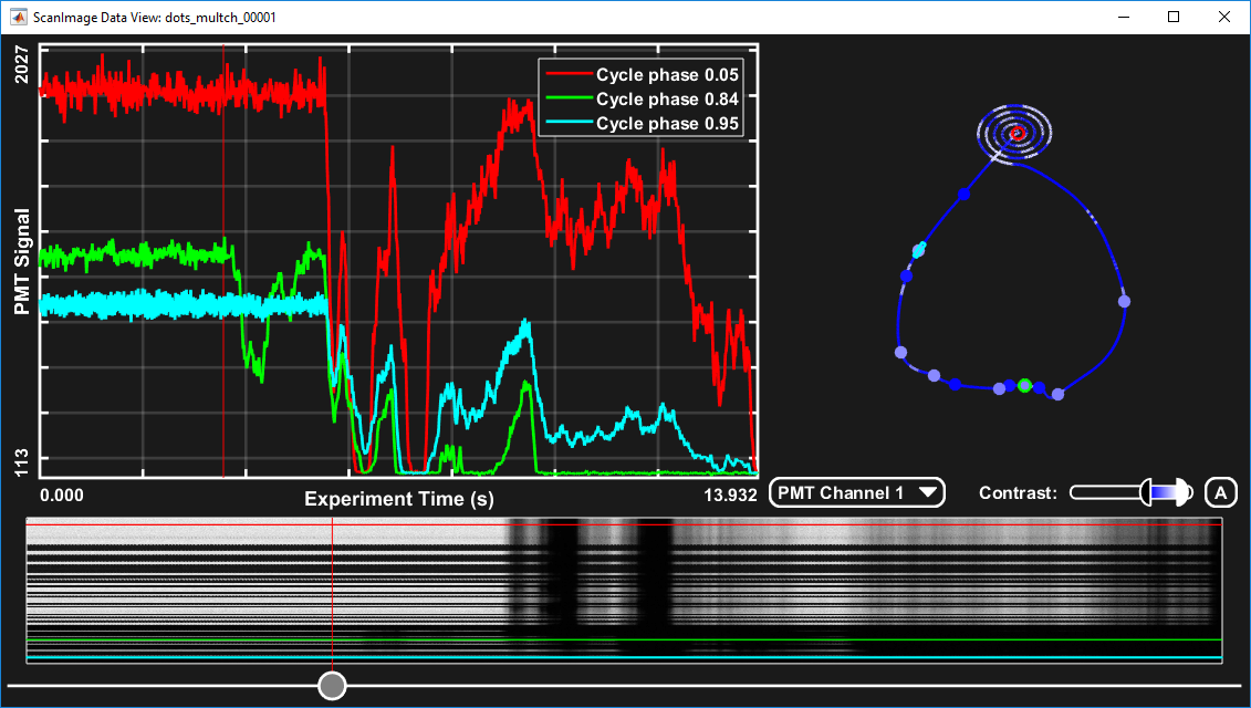
Analysis
Starting in SI Premium 2018a and SI 5.4 , the Offline Data Viewer is an option for analyzing data acquired from a previous acquisition. The tool allows you to easily create plots to show the change in fluorescence over time for a given pixel or area.
It is accessed via command window by execucting the command:
1>> sidataview
Learn more about SIDataView