FOV Curvature Correction

FOV curvature can be addressed now through a miscellaneous device added to the configuration, display, and controls. This can be used either for

correction of the curvature of the field of view, or
addition of curvature to the FOV to image more ROIs per individual frame

It works by using a paired fastZ device to vary the depth of the focal point as a function of XY positiion in the FOV. Care must be taken to scan at rates that accommodate the performance of the paired fastZ device.

Note

There was and still exists an old, similar, but undocumented means for correcting for FOV curvature and it does not incorporate a helpful GUI. This is available in both basic and premium ScanImage. To use it, ellipsoid semi-axes lengths must be input from the machine data file and the handle to the FastZ component hSI.hFastZ must have its enableFieldCurveCorr property set to true from the command window.

Do not place a check in the Correct Field Curvature checkbox if you are using this legacy version of the feature.

Configuration

In ScanImage, open the Resource configuration window from the launch window or from the Main Controls window under File>Configuration.

From the Resource Configuration window, click the + button. Select Miscellaneous from the sidebar, and select the Thorlabs Liquid Crystal Analog FastZ device from the list of devices. Click Add.
A window like shown below should appear. Below is a description of each of the configuration parameters

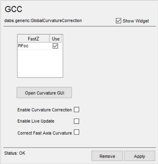
FastZ Table	Select the FastZ actuators that should be controlled by this curvature correction device.
Open Curvature GUI	Once ScanImage has been launched, the curvature of the FOV can be defined in the GUI launched by clicking this button. The GUI can also be launched by clicking the image in the widget.
Enable Curvature Correction	If checked, subsequent acquisitions will apply the curvature settings defined in the GUI to the selected fastZ actuator’s analog output buffer thus correcting for or adding field curvature.
Enable Live Update	If checked, then the analog output buffer can be recalculated while in the middle of an acquisition if the analog output buffer is small enough that it makes sense to attempt live updating (less than 3e6 samples). Note The number of samples of an acquisition is equal to the sample rate for tasks multiplied by the duration of a frame for a planar acquisition or the duration of the volume for fast stack acquisition
Correct Curvature within Resonant Period	If checked and the imaging scanner is configured for resonant scanning, the curvature is corrected within the resonant period.

GUI

The GUI is subdivided into 3 parts:

Axes
Settings Panel
Sliders

Axes

The axes are plotted in microns in each of XYZ and display 4 things:

Control Surface - The light blue surface used to define curvature at key Zs. Alpha of this surface can be controlled with the Control Surface Alpha slider
Scan Bounds - The part of sample space that can be scanned
Scanfields - The scanfields as they are currently configured for the next grab or loop acquisition. Scanfield colors can be selected by clicking the Colors button beside its corresponding checkbox.
Last Image - The last planar or stack image data acquired. Stacks are imported as flat planes at the sample Zs they were acquired at. This takes on the color configured as the merge color from the Channels window. This is plotted with alpha controlled by the Last Image Alpha Map slider

The visibility of each can be toggled from its corresponding checkbox.

The mouse controls for the axes are: - Scroll - zoom in and out - Left click and drag - pan - Middle click or Shift and left click and drag - Orbit

There is also a histogram to alter the constrast, alpha, color, etc of most recently acquired image data.

Settings Panel

The table contains all the curvature data for each key Z. The cells of the table are editable except for the key Z. Clicking a table cell renders the Control Surface at the depth of the cell’s corresponding key Z. Clicking the X at the last column deletes the row.

The save and load buttons save and load the curvature data displayed in the table.

The Add Point Cloud to Z and Determine Sample Tilt buttons are specialized functions.

A simple way to quickly characterize the curvature of the imaging system is to image a stack at the interface of the optical medium (air/water) and a flat fluorescent sample using a sample stage or similar to navigate to each slice. The surface given by the max projection in Z of this stack can be assumed to be the top of the flat, fluorescent sample. After taking the stack, you can click Add Point Cloud to Z to acquire such a max projection surface and use it to define the surface used to scan.

Note

A sample stage should be used for this max projection especially if that fastZ device you use is expected to have different field curvature throughout its range of motion.

If using a headfixed headbar, it may be useful to determine the tilt of the headbar relative to the optical axis of the microscope. For this, one mount a sample with a thin coating of fluorescent ink and grab a stack traversing the whole thickness of the ink. Then you can open the Global Curvature Correction GUI, check the Last Image checkbox, and then click the Determine sample tilt button to automatically fill in the azimuth and elevation values to match the tilt of the sample.

The FastZ target position [um] is the fastZ position used to define a key surface. The fastZ target position for an plane acquisition or slice of a stack is used to determine the curvature at that plane.

Sliders

The sliders are a means to help define the curvature at each key Z.

X Axis	Semi-Axis Length in X of the ellipsoid used to define the control surface.
Y Axis	Length of the Y Axis of the ellipsoid used to define the control surface.
Z Axis	Length of the Z Axis of the ellipsoid used to define the control surface.
Sweep [deg]	Angle from the Z axis to the outer edge of the ellipse. When adjusting elevation, this is automatically adjusted to prevent multiple zs per XY location.
Azimuth [deg]	The azimuthal angle - angle measured from the reference positive X axis to the X axis of the ellipsoid.
Elevation [deg]	The angle of elevation from the horizontal to the key surface tangent at the surface center point.
X Offset [um]	The offset of the ellipsoid in the reference X direction.
Y Offset [um]	The offset of the ellipsoid in the reference Y direction.
Z Offset [um]	The offset of the ellipsoid in the reference Z direction.

Use

For each fastZ position that a planar acquisition or stack acquisition slice can be made, we aim to shape the curvature of that plane or slice uniquely with this GUI. Given that fastZ actuators are typically driven by analog waveforms, that means that there is a continuum of fastZ positions in the range of the actuator. Thus, one can define the curvature at several key fastZ positions, and then for any fastZ positions not defined, the curvature settings from the nearest key Zs.

Defining the curvature at any one key Z can be done via dragging sliders in the right pane of the GUI.

Correcting for field curvature involves iteratively acquiring a stack of a known flat fluorescent sample (glass slide with highlighter ink smeared thin over top) without field curvature compensation, defining the curvature at such a depth, moving a Z-stage by some sub-multiple of the fastZ range, and repeating the process for several key depths. The process is done in the tutorial for a single surface, however to map a mostly flat field of view to a curved surface.

Note

In the video, the stack is acquired with the fastZ device located towards the bottom of its travel range.

Also in the video, the max projection z surface data was used for key Z = 115 µm, i.e. not at the bottom of the travel range.

In the case of this video, it was not very detrimental given the extreme curvature of the insect eye, but ideally, the key Z used for the surface matches the fastZ actuator Z used throughout the stage-mediated stack used to acquire that max projection surface.

This is (again) because the fastZ device can exhibit different curvature at different fastZ positions, particularly in the case of remote focus fastZs.

Tutorial

The feature tutorial video at the top shows how the device can be used to image a plane mapped to the curvature of the eye of an insect. It is performed on a microscope equipped with the RMR scanhead and a piezo objective stage.

First a stack is taken without any correction. Then a galvo-galvo scan is performed to precisely follow the curvature for all points in the scanfield.

below is a sample script to try this yourself with sample of your choice.

Script

ACQUIRE WITHOUT CURVATURE CORRECTION

Start with Resonant, 512x512 30Hz
Disable curvature correction
Focus
10 frames averaging
Bring focal point through fastZ range
Enable Stack - Bounded 5 frame per slice, 50 slices, 10 volumes, slow stack
Grab

DEFINING AND APPLYING CURVATURE CORRECTION WITH LINEAR SCANNING

open GCC GUI
get context stack, set contrast
Add Point Cloud to Z using the max projection of the slow stack just acquired
To slow down the acquisition to accommodate speed of fastZ device and also to maintain reasonable control waveform buffer sizes: - Set desired control sample rate to 10 kHz from RggScan’s advanced tab in the resource configuration -> lower control sample rate -> takes less time to optimize or start acquisitions - Set pixel bin factor higher -> increase scanning time -> easier for fastZ to scan - Set sample rate lower -> increase scanning time -> easier for fastZ to scan - Lower frame pixel resolution -> less pixels to scan, scan frames faster but -> less control samples to generate -> takes less time to optimize/start acquisitions
Switch to linear scanning
Disable stack
Enable GCC
Set FastZ Target position to overlap eye
Open Waveform Controls Tab, go to Z tab, optimize waveforms
Focus

APPLYING CURVATURE CORRECTION WITH MROI SCANNING 8:20

Go back to Resonant
Configure GCC device not to try to correct z along the fast (resonant) axis
Change desired control sample rate to 1000 kHz
Get context image
enable MROI
Add ROIs that are not too tall and centered.
Set flyto and flyback time to 20 ms
Show scanfields in Curvature Correction tab
Open Waveform Controls Tab and optimize Z waveforms.
Focus with MROI.

Caveats

Even with an idealized fastZ actuator with infinitesimally short duration step times, the max sample rate of the fastZ task will limit the number of samples that can be fit into a line. For the vDAQ, for instance, the max sample rate that can be used for the fastZ task is 1 MHz (specified from the Advanced tab of the RggScan configuration page). This limitation would only be noticable for the resonant scan mode. For example, 1 MHz sample rate in an acquisition with an 8 kHz resonant scanner with a temporal fill fraction of 0.7192 and bidirectional acquisition of lines yields 1e6 / (2*8e3) * 0.7192 = 44 samples, or 29 samples for a 12 kHz resonant mirror. For an ellipsoid representing the curvature, this should be more than enough. This does make more complicated surfaces less feasible.

FastZ devices at the time of publishing this cannot support high bandwidth scanning in the z dimension. Those that do may suffer from hysteresis.

Tip

It may be helpful for imaging systems with paired gcc fastZs suffering from hysteresis to separate even and odd lines of bidirectionally (X) scanned frames into their own images for analysis as hysteresis has them imaging slightly distinct surfaces if the surfaces being scanned by the gcc are tilted such that they are lower on the left/right side than the right/left side.